Many distance-based machine learning algorithms are general enough that we can change the way we compute the distance between two points. When we look at data in $\mathbb{R}^n$, for $n\in\mathbb{N}^*$, we are used to the euclidean distance. This distance measures the length of the straight line connecting the two points, as a kind of generalization of the Pythagorean theorem.
Vários algoritmos de aprendizado de máquina baseados em distância são genéricos o suficiente para mudarmos a forma como calculamos a distância entre dois pontos. Quando olhamos para dados em $\mathbb{R}^n$, para $n\in\mathbb{N}^*$, estamos acostumados com a distância euclidiana. Essa distância calcula o tamanho do comprimento de reta que liga os dois pontos, com uma espécie de generalização do teorema de Pitágoras.
Explicitly, for $\textbf{x} = (x_1, x_2, \cdots, x_n) \in \mathbb{R}^n$ and $\textbf{y} = (y_1, y_2, \cdots, y_n) \in \mathbb{R}^n$, the distance is given by
Explicitamente temos, para $\textbf{x} = (x_1, x_2, \cdots, x_n) \in \mathbb{R}^n$ e $\textbf{y} = (y_1, y_2, \cdots, y_n) \in \mathbb{R}^n$, a distância dada por
\[\begin{equation*} \textrm{euclidean distance between }\textbf{x}\textrm{ and }\textbf{y} = \sqrt{ \sum_{i=1}^{n} |x_i-y_i|^2 } . \end{equation*}\]
\[\begin{equation*} \textrm{distância euclidiana entre }\textbf{x}\textrm{ e }\textbf{y} = \sqrt{ \sum_{i=1}^{n} |x_i-y_i|^2 } . \end{equation*}\]
However, depending on the nature of the problem, this distance may not be the most appropriate one. In this post, we will discuss the definition of distance through the lens of basic concepts from the topology of metric spaces, and illustrate some classic metrics while understanding the differences between them. This discussion can be important for going deeper into classic algorithms that rely on a distance computation, such as k-NN, DBScan, and K-Means and its variations. It also helps you learn to recognize other moments when you can use the concept of distance.
Entretanto, dependendo da natureza do problema essa distância pode não ser a mais indicada. Neste post, vamos conversar sobre a definição de distância aos olhos de conceitos básicos de topologia de espaços métricos e exemplificar algumas métricas clássicas entendendo a diferença entre elas. Essa discussão pode ser importante para se aprofundar em algoritmos clássicos que utilizam um cálculo de distância como o k-NN, o DBScan e o K-Means e suas variações. Além de aprender a identificar outros momentos em que você pode utilizar o conceito de distância.
Defining the distance between two points formally
Definindo formalmente a distância entre dois pontos
Intuitively, a distance must satisfy some properties that arise from the way we intuitively perceive distance. We will see a mathematical definition for it that tries to synthesize these notions in mathematically clear terms.
Intuitivamente, uma distância precisa satisfazer algumas propriedades que surgem da forma como vemos distância intuitivamente. Iremos ver uma definição matemática para ela que tenta sintetizar essas noções em termos matematicamente claros.
First, it is reasonable to ask for symmetry: the distance from $x$ to $y$ should equal the distance from $y$ to $x$. This seems obvious, but our formal definition of distance will be a function that takes two inputs and returns a value, which we will call the distance between the input arguments. This first desired property tells us that the order in which we provide the inputs does not matter.
Primeiro, é razoável pedir simetria: a distância de $x$ até $y$ seja igual à distância de $y$ até $x$. Isso parece óbvio, mas a nossa definição formal de distância será uma função que aceita duas entradas e retorna um valor, que chamaremos de distância entre os argumentos de entrada. Essa primeira propriedade desejada nos dirá que não importa a ordem em que damos as entradas.
Another desirable property is identity: the distance from a point to itself is zero, and if two points are at distance zero then they are the same element. This is also quite reasonable and tells us that only the point itself is at distance zero from itself.
Uma outra propriedade desejável é a identidade: a distância de um ponto até ele mesmo é zero e se dois pontos estão a uma distância zero então eles são o mesmo elemento. Isso também é bem razoável e nos diz que apenas o próprio ponto tem distância zero dele mesmo.
Finally, in middle school we are told that, given a triangle, the sum of the lengths of two sides is always greater than or equal to the length of the remaining side for the triangle to be valid. We will want to keep this property in our formal definition of distance, calling it the triangle inequality.
Por fim, no ensino fundamental nos dizem que, dado um triângulo, então a soma dos comprimentos de dois lados sempre é maior ou igual ao comprimento do lado restante para o triângulo ser válido. Vamos querer manter essa propriedade na nossa definição formal de distância, chamando essa propriedade de desigualdade triangular.
With this intuitive notion of distance, we create the formalization given by the mathematical definition:
Com essa noção intuitiva de distância, criamos a formalização dada pela definição matemática:
Definition: Given a set $\mathcal{A}$, a function $d:\mathcal{A}\times\mathcal{A}\to \mathbb{R}$ is called a metric (or distance) on $\mathcal{A}$ if, for any $x,y,z\in\mathcal{A}$, it satisfies:
Definição: Dado um conjunto $\mathcal{A}$, uma função $d:\mathcal{A}\times\mathcal{A}\to \mathbb{R}$ é chamada de uma métrica (ou distância) em $\mathcal{A}$ se, dados $x,y,z\in\mathcal{A}$ quaisquer, satisfaz:
- $d(x,y) = 0 \Leftrightarrow x = y$ (identity);
- $d(x,y) = d(y,x)$ (symmetry);
- $d(x,y) + d(y,z) \geq d(x,z)$ (triangle inequality).
- $d(x,y) = 0 \Leftrightarrow x = y$ (identidade);
- $d(x,y) = d(y,x)$ (simetria);
- $d(x,y) + d(y,z) \geq d(x,z)$ (desigualdade triangular).
Note that from these properties we can derive other desired properties, such as non-negativity. It would be counterintuitive to measure the distance between two points and obtain a negative number. To show that this holds in our case, that is, that $d(x,y)\geq 0$ for any $x,y\in \mathcal{A}$, we use the triangle inequality: $d(x,y) + d(y,x) \geq d(x,x)$. By symmetry and using that $d(x,x)=0$, we have $2 \, d(x,y) \geq 0$, and we conclude what we wanted.
Repare que dessas propriedades, tiramos ainda outras propriedades desejadas, como, por exemplo, a não-negatividade. Seria contraintuitivo medir a distância entre dois pontos e obter um número negativo. Para mostrar que isso vale no nosso caso, ou seja, que $d(x,y)\geq 0$ para quaisquer $x,y\in \mathcal{A}$, usamos a desigualdade triangular: $d(x,y) + d(y,x) \geq d(x,x)$. Pela simetria e usando que $d(x,x)=0$ temos que $2 \, d(x,y) \geq 0$, e concluímos o desejado.
We define that, given a metric function $d$ as above, the distance between two points $x,y\in \mathcal{A}$ is given by $d(x,y)$.
Definimos que, dada uma função métrica $d$ como anteriormente, a distância entre dois pontos $x,y\in \mathcal{A}$ é dada por $d(x,y)$.
Classic examples for $\mathbb{R}^n$
Exemplos clássicos para $\mathbb{R}^n$
The nature and choice of the metric vary according to the problem being studied. In general, when $\mathcal{A}=\mathbb{R}^n$, we are interested in distances induced by the Lp norms (with $1\leq p \leq \infty$) given in the form
A natureza e escolha da métrica varia de acordo com o problema estudado. Em geral, quando $\mathcal{A}=\mathbb{R}^n$, estamos interessados em distâncias induzidas pelas normas Lp (com $1\leq p \leq \infty$) dadas na forma
with coordinate-wise vector operations, where the Lp norm $||\cdot||_p : \mathbb{R}^n \to \mathbb{R} $ is given by
com soma de vetores coordenada a coordenada em que a norma Lp $||\cdot||_p : \mathbb{R}^n \to \mathbb{R} $ é dada por
In the machine learning context, the metrics in this family of distances are better known as the Minkowski distance with parameter p. Note that the usual euclidean distance is the Minkowski distance with parameter 2. In the limiting case, when $p=\infty$, the norm is defined as the largest absolute value among the coordinates, that is,
As métricas dessa família de distâncias, no contexto de aprendizado de máquina, são mais conhecidas como distância Minkowski com parâmetro p. Repare que a distância euclidiana usual é a distância de Minkowski com parâmetro 2. O caso limite, quando $p=\infty$, é definido como o maior valor absoluto entre as coordenadas, ou seja,
The metric $d_\infty$ is also known as the Chebyshev distance or maximum distance. Another classic name for the metric $d_1$ is the Manhattan distance.
A métrica $d_\infty$ é também conhecida como distância de Chebyshev ou do máximo. Um outro nome clássico para a métrica $d_1$ é distância de Manhattan.
Different balls of $\mathbb{R}^n$
Diferentes bolas do $\mathbb{R}^n$
To illustrate how these different ways of measuring distance work, let us define a fundamental concept from the topology of metric spaces: the open ball. The notion of a ball tries to give meaning to the question: "What does it mean for an element to be close to another?".
Para ilustrar como essas diferentes formas de medir distância funcionam, vamos definir um conceito primordial de topologia de espaços métricos: a bola aberta. A noção de bola tenta dar um significado para a pergunta: "O que significa ter um elemento perto de outro?".
First, we will have a parameter related to the central point of comparison. This will be the element against which we compare the others, trying to answer whether they are close or not. Moreover, the meaning of close depends on our tolerance: two people sitting less than 1 meter apart is close (even more so in coronavirus times), but a meteor 1 kilometer from Earth is also close in the eyes of an astronomer. Our ball will also have a parameter, which we will call the radius, which tells us up to what point we are considering close.
Primeiro, teremos um parâmetro relacionado com o ponto central de comparação. Este será o elemento com o qual compararemos os outros, tentando responder se estão próximos ou não. Além disso, o significado de perto depende da nossa tolerância: duas pessoas sentadas a menos de 1 metro é perto (ainda mais em época de coronavírus), mas um meteoro a 1 quilômetro da Terra também é perto aos olhos de um astrônomo. A nossa bola também terá um parâmetro, que chamaremos de raio, que nos dará até quanto estamos considerando perto.
Definition: Let $d$ be a metric on a set $\mathcal{A}$. An open ball of radius $r>0$ centered at the point $x\in \mathcal{A}$ is the set
Definição: Seja $d$ uma métrica em um conjunto $\mathcal{A}$. Uma bola aberta de raio $r>0$ centrada no ponto $x\in \mathcal{A}$ é o conjunto
The elements of $B_d(x;r)$ are the elements of $\mathcal{A}$ close to $x$ (under this radius-$r$ tolerance). This notion of closeness, formalized by the ball, helps define the meaning of convergence and continuity in abstract spaces, but we will not get into those topics.
Os elementos de $B_d(x;r)$ são os elementos de $\mathcal{A}$ perto de $x$ (sob essa tolerância de raio $r$). Essa noção de perto, formalizada pela bola, ajuda a definir o significado de convergência e continuidade em espaços abstratos, mas não entraremos nesses tópicos.
Let us play with the shape of these balls when $\mathcal{A}=\mathbb{R}^2$ and $d=d_p$, the Minkowski distance with parameter $p$, varying the value of $p$. These metrics are already implemented in
sklearn.metrics.DistanceMetric; we will just create a function that takes a metric, a radius, and a center, and plots the associated ball.Vamos brincar com o formato dessas bolas quando $\mathcal{A}=\mathbb{R}^2$ e $d=d_p$, a distância de Minkowski de parâmetro $p$, variando o valor do $p$. Essas métricas já estão implementadas no
sklearn.metrics.DistanceMetric, vamos apenas criar uma função que recebe uma métrica, um raio e um centro, e plota a bola associada.from sklearn.metrics import DistanceMetric
def open_ball(metrics, radius=1, center=[0, 0], titles=None):
"""Plot the unit balls (up to three per row) of the metrics in `metrics`.
metrics: list of sklearn.metrics.DistanceMetric objects.
radius: ball radius (float) or a list of radii, one per metric.
center: shared center of the balls, [x, y]. Axes always between -1.5 and 1.5.
titles: optional list of subplot titles, one per metric.
"""
if type(radius) in [int, float]:
radius = [radius] * len(metrics)
# grid used to draw the level curve of the indicator function
# (which tells whether the point is inside or outside the ball)
x_vals = np.linspace(-1.5, 1.5, 400)
y_vals = np.linspace(-1.5, 1.5, 400)
X, Y = np.meshgrid(x_vals, y_vals)
n = len(metrics)
m = int(np.ceil(len(metrics) / 3))
plt.figure(figsize=(12, 4 * m))
for j, metric in zip(range(1, n + 1), metrics):
plt.subplot(m, 3, j)
# indicator function: 1 if the point is inside the ball, 0 otherwise
Z = np.asarray(
[
[
1
if metric.pairwise(np.array([[x, y]]), np.array([center]))[0, 0] < radius[j - 1]
else 0
for x in x_vals
]
for y in y_vals
]
)
plt.contourf(X, Y, Z, levels=[-0.1, 0.1, 0.9, 1.1], cmap=cmap)
plt.xticks([-1, 0, 1])
plt.yticks([-1, 0, 1])
if titles is not None:
plt.title(titles[j - 1])
The plots below show how the shape of the ball centered at the origin with radius 1 varies for $p = 1$, $1.5$, $2$, $3$, $10$, $\infty$, in order.
Os plots abaixo mostram como varia o formato da bola centrada na origem e de raio 1 para $p = 1$, $1.5$, $2$, $3$, $10$, $\infty$, em ordem.
ps = [1, 1.5, 2, 3, 10]
metrics = []
for p in ps:
    metrics.append(DistanceMetric.get_metric("minkowski", p=p))
metrics.append(DistanceMetric.get_metric("chebyshev"))

titles = [f"$p = {p}$" for p in ps] + [r"$p = \infty$"]
open_ball(metrics, titles=titles)
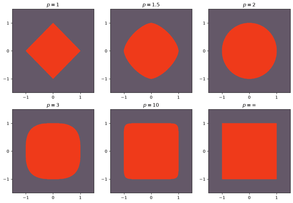
The boundary of our ball is not included in it, hence the name open, analogous to the open intervals of the real line that do not contain the boundary elements (indeed, an open interval is an open ball on the line). In any case, it is interesting to analyze the boundary to understand its different shapes. Since we have $r=1$ and the center as the origin, the boundary is given by the values $(x_1,x_2)\in\mathbb{R}^2$ that satisfy the equation
A borda da nossa bola não está incluída nela, daí o nome aberta, análogo aos intervalos abertos da reta que não contêm os elementos da fronteira (de fato, um intervalo aberto é uma bola aberta na reta). De toda forma é interessante analisar a borda para entender seus diferentes formatos. Como temos $r=1$ e o centro como sendo a origem, vale que a borda é dada pelos valores $(x_1,x_2)\in\mathbb{R}^2$ que satisfazem a equação
When $p=2$, we get the circle, from our euclidean notion of a ball. But note that when $p=1$, we get four straight lines, depending on the sign of $x_1$ and $x_2$, and that is why we obtain the diamond. The case $p=\infty$ is given by
Quando $p=2$, temos o círculo, da nossa noção euclidiana de bola. Mas repare que quando $p=1$, temos quatro retas, dependendo do sinal de $x_1$ e $x_2$ e por isso obtemos o losango. O caso $p=\infty$ é dado por
and that is why the boundary lies at the points where $|x_1|=1$ or $|x_2|=1$.
e é por isso que temos a borda nos valores dos pontos que tem $|x_1|=1$ ou $|x_2|=1$.
I will never understand what is funny about the show El Chavo, but it is impossible not to make an unfortunate comment about how Kiko's square balls are actually using the Chebyshev metric. Kiko, like you now, understands quite a bit about the topology of metric spaces.
Eu nunca vou entender qual a graça do programa Chaves, mas impossível não fazer um comentário infeliz sobre as bolas quadradas do Kiko estarem na verdade utilizando a métrica de Chebyshev. O Kiko, como você agora, entende bastante de topologia de espaços métricos.
More examples
Mais exemplos
Let us go through a few more interesting examples that can help build intuition or that are relevant in the data science context.
Vamos passar por mais alguns exemplos interessantes que podem ajudar a construir a intuição ou que são relevantes no contexto de ciência de dados.
Discrete metric
Métrica discreta
Imagine an exotic experiment in which the explicit value of the distance between two points is not important, but it is relevant to know whether two elements are equal or not. In this scenario, the discrete metric can be useful. Given any $\mathcal{A}$, the distance $d_{\textrm{disc}}$ between $x,y\in\mathcal{A}$ is given by
Imagine um experimento exótico em que o valor explícito da distância entre dois pontos não é importante, mas é relevante saber se dois elementos são iguais ou não. Nesse cenário, a métrica discreta pode ser útil. Dado $\mathcal{A}$ qualquer, a distância $d_{\textrm{disc}}$ entre $x,y\in\mathcal{A}$ é dada por
\[\begin{equation*} d_{\textrm{disc}}(x,y)= \begin{cases} 0 \textrm{, if }x=y,\\ 1 \textrm{, otherwise.} \end{cases} \end{equation*}\]
\[\begin{equation*} d_{\textrm{disc}}(x,y)= \begin{cases} 0 \textrm{, se }x=y,\\ 1 \textrm{, caso contrário.} \end{cases} \end{equation*}\]
It is a nice exercise to convince yourself that this form of distance satisfies the properties we wanted in the definition of a metric.
É um exercício legal se convencer que esta forma de distância satisfaz as propriedades que desejávamos na definição de métrica.
Here, the notion of close or far becomes a bit counterintuitive. If $\mathcal{A}=\mathbb{R}^2$, then the point $(0,0)$ is at the same distance from the point $(0,1)$ and from the point $(42,-42)$. We can see this by analyzing the balls for different values of the radius $r$. For any $r\in (0,1]$, we have that $B_{d_{\textrm{disc}}}(x;r) = \{ x \}$, since only $x$ is at a distance less than 1 from itself. Now, for any $r\in (1,\infty)$ we have that $B_{d_{\textrm{disc}}}(x;r) = \mathcal{A}$, since every point is at a distance less than or equal to 1 from $x$.
Aqui, a noção de perto ou distante se torna um pouco contraintuitiva. Se $\mathcal{A}=\mathbb{R}^2$, então o ponto $(0,0)$ está a mesma distância do ponto $(0,1)$ e do ponto $(42,-42)$. Podemos olhar isso analisando as bolas para diferentes valores do raio $r$. Para qualquer $r\in (0,1]$, temos que $B_{d_{\textrm{disc}}}(x;r) = \{ x \}$, pois somente $x$ está a uma distância menor que 1 dele mesmo. Agora, para qualquer $r\in (1,\infty)$ temos que $B_{d_{\textrm{disc}}}(x;r) = \mathcal{A}$ uma vez que qualquer ponto está a uma distância menor ou igual a 1 de $x$.
In
sklearn.metrics.DistanceMetric, we can pass a generic metric that respects the formal definition we made. We use the pyfunc argument and set the metric function in func, which takes two one-dimensional numpy vectors and returns the distance between them.No
sklearn.metrics.DistanceMetric, podemos passar uma métrica genérica que respeite a definição que fizemos na definição formal. Usando o argumento pyfunc e estabelecendo a função métrica em func que recebe dois vetores numpy unidimensionais e retorna a distância entre eles.def discrete(X, Y):
"""Discrete distance between X and Y: 0 if they are equal, 1 otherwise."""
if np.all(X == Y):
return 0
else:
return 1
open_ball([DistanceMetric.get_metric("pyfunc", func=discrete)] * 2, [0.5, 1.5])
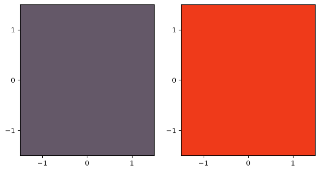
In the figure below, we pass the values $0.5$ and $1.5$ as the radii of the balls, to see the effect discussed earlier that $B_{d_{\textrm{disc}}}((0,0);0.5)=\{(0,0)\}$ and $B_{d_{\textrm{disc}}}((0,0);1.5)=\mathbb{R}^2$.
Na figura abaixo, passamos como raios das bolas os valores $0.5$ e $1.5$, para ver o efeito discutido anteriormente de que $B_{d_{\textrm{disc}}}((0,0);0.5)=\{(0,0)\}$ e $B_{d_{\textrm{disc}}}((0,0);1.5)=\mathbb{R}^2$.
Hamming distance
Distância de Hamming
The Hamming distance between two vectors of size $n$ is the number of components that differ between them. It turns out to be very useful when the component values are not numeric or have no sense of order. Let us give a scenario in which it can make sense to use it:
A distância de Hamming entre dois vetores de tamanho $n$ é o número de componentes diferentes entre eles. Ela se demonstra muito útil quando os valores das componentes não são numéricos ou não têm um sentido de ordem. Vamos dar um cenário em que pode fazer sentido usá-la:
Distance between pots
Distância entre panelas
Imagine I want to describe the distance between two pots, and the attributes I consider important about this object are the color and whether or not it has a handle. In this case, we represent our space as $\mathcal{A} =$ $\{ \textrm{gray}, \textrm{red}, \textrm{black} \}$ $\times \{\textrm{has handle}, \textrm{no handle} \}$. A pot is represented by a two-component vector: the first is its color and the second the presence of a handle, for example $(\textrm{gray}, \textrm{has handle})$.
Imagine que eu queira descrever a distância entre duas panelas e os atributos que eu considero importante sobre esse objeto são a cor e a presença ou não de cabo. Neste caso, estamos representando nosso espaço como $\mathcal{A} =$ $\{ \textrm{cinza}, \textrm{vermelha}, \textrm{preta} \}$ $\times \{\textrm{tem cabo}, \textrm{não tem cabo} \}$. Uma panela é representada por um vetor de duas componentes, na primeira a sua cor e na segunda a presença de cabo, por exemplo $(\textrm{cinza}, \textrm{tem cabo})$.
The way we have seen distance so far only talked about numbers. We can adapt $\mathcal{A}$ to analyze the space $\mathcal{A}' =\{1,2,3\}\times\{1,2\}$, where we make a bijection between the elements through the map ($\textrm{gray}\to 1$, $\textrm{red}\to 2$, $\textrm{black}\to 3$) and ($\textrm{has handle}\to 1$, $\textrm{no handle}\to 2$). With this transformation, we can use, for example, the Minkowski distance with parameter 1.
A maneira como vimos distância até agora apenas falava sobre números. Podemos adaptar $\mathcal{A}$ para analisar o espaço $\mathcal{A}' =\{1,2,3\}\times\{1,2\}$ em que fazemos a bijeção entre os elementos pelo mapa ($\textrm{cinza}\to 1$, $\textrm{vermelha}\to 2$, $\textrm{preta}\to 3$) e ($\textrm{tem cabo}\to 1$, $\textrm{não tem cabo}\to 2$). Com essa transformação, podemos usar por exemplo a distância de Minkowski com parâmetro 1.
Imagine we have $\textrm{pot}_1 = (\textrm{gray},\textrm{has handle})$, $\textrm{pot}_2 = (\textrm{black},\textrm{has handle})$, and $\textrm{pot}_3 = (\textrm{red},\textrm{no handle})$. In this case, we would get things like:
Imagine que temos $\textrm{panela}_1 = (\textrm{cinza},\textrm{tem cabo})$, $\textrm{panela}_2 = (\textrm{preta},\textrm{tem cabo})$, e $\textrm{panela}_3 = (\textrm{vermelha},\textrm{não tem cabo})$. Neste caso, ficaríamos com coisas do tipo:
\[\begin{aligned} d_{\textrm{pots}}(\textrm{pot}_1, \textrm{pot}_2 ) &= d_1((1,1),(3,1)) = |1-3|+|1-1| = 2,\\ \textrm{while}\quad d_{\textrm{pots}}(\textrm{pot}_1, \textrm{pot}_3 ) &= d_1((1,1),(2,2)) = |1-2|+|1-2| = 2. \end{aligned}\]
\[\begin{aligned} d_{\textrm{panelas}}(\textrm{panela}_1, \textrm{panela}_2 ) &= d_1((1,1),(3,1)) = |1-3|+|1-1| = 2,\\ \textrm{enquanto}\quad d_{\textrm{panelas}}(\textrm{panela}_1, \textrm{panela}_3 ) &= d_1((1,1),(2,2)) = |1-2|+|1-2| = 2. \end{aligned}\]
This way of computing distances is telling us that $\textrm{pot}_1$ is at the same distance from $\textrm{pot}_2$ and from $\textrm{pot}_3$. $\textrm{pot}_1$ differs from $\textrm{pot}_2$ only by color, while it differs in color and in the presence of a handle from $\textrm{pot}_3$. The problem arose here because we mapped the colors onto the line as if these objects had an order, which does not make sense here.
Esta forma de calcular distâncias, está nos falando que a $\textrm{panela}_1$ está a mesma distância da $\textrm{panela}_2$ e da $\textrm{panela}_3$. A $\textrm{panela}_1$ difere da $\textrm{panela}_2$ apenas pela cor, enquanto difere em cor e na presença de cabo da $\textrm{panela}_3$. O problema surgiu aqui porque levamos as cores pra reta como se esses objetos tivessem uma ordem, o que não faz sentido aqui.
An alternative is precisely to compute the Hamming distance of the pots, adding $1$ to the distance for each category (color and presence of a handle) in which they differ. In this case, the Hamming distance between $\textrm{pot}_1$ and $\textrm{pot}_2$ would be 1, since they differ only in the first component.
Uma alternativa é justamente calcular a distância Hamming das panelas, somando $1$ na distância pra cada categoria (cor e presença de cabo) em que há diferença. Neste caso a distância de Hamming da $\textrm{panela}_1$ e a $\textrm{panela}_2$ seria 1 pois diferem apenas na primeira componente.
$\oint$ The Hamming distance is equivalent to applying a
sklearn.preprocessing.OneHotEncoder to each of the vector components and then computing the distance with any Minkowski (dividing the final result by 2).$\oint$ A distância de Hamming é equivalente a fazer um
sklearn.preprocessing.OneHotEncoder de cada uma das componentes dos vetores e depois calcular a distância com qualquer Minkowski (dividindo por 2 o resultado final).Angular distance
Distância do ângulo
Imagine that $\mathcal{A}= S^{\,1} =\{ (a,b)\in\mathbb{R}^2 : a^2 + b^2 = 1 \}$, that is, we are looking exactly at the plane vectors with L2 norm equal to 1, the traditional circle we know. We can define an angular distance given by the angle between two points. For example, the distance between $(0,1)$ and $(1,0)$ would be $\pi/2$, since the angle between these two vectors is $90^\circ$. An explicit way to compute this angle is
Imagine que $\mathcal{A}= S^{\,1} =\{ (a,b)\in\mathbb{R}^2 : a^2 + b^2 = 1 \}$, ou seja, estamos olhando exatamente para os vetores do plano de norma L2 igual a 1, o círculo tradicional que conhecemos. Podemos definir uma distância do ângulo dada pelo ângulo entre dois pontos. Por exemplo, a distância entre $(0,1)$ e $(1,0)$ seria $\pi/2$, uma vez que o ângulo entre estes dois vetores é $90^\circ$. Uma forma explícita de calcular esse ângulo é
where the argument of the arccosine is precisely the inner product between the vectors.
em que o argumento do arco cosseno é justamente o produto interno entre os vetores.
It is important to note that we restricted ourselves to looking only at vectors of size $1$ in order to satisfy the definition of a metric we made. Looking at the angle between vectors of arbitrary size does not give us a metric, because we do not have the identity property: the angle between the vectors $(1,0)$ and $(2,0)$ is $0$, yet $(1,0)\neq (2,0)$. Moreover, it is not possible to define the angle between an arbitrary vector and the zero vector.
É importante reparar que fizemos a restrição de olhar apenas para vetores de tamanho $1$ pra satisfazer a definição de métrica que fizemos. Olhar o ângulo entre vetores de tamanho qualquer não nos dá uma métrica pois não temos a propriedade de identidade: o ângulo entre os vetores $(1,0)$ e $(2,0)$ é $0$ entretanto $(1,0)\neq (2,0)$. Além disso, não é possível definir o ângulo entre um vetor qualquer e o vetor nulo.
We can generalize this distance to vectors in higher dimensions on the surface of a unit hypersphere $\mathcal{A} = S^{\,n-1} = \{ \textbf{x}\in\mathbb{R}^n : ||\textbf{x}||_2 = 1 \}$. We compute the distance between $\textbf{x} = (x_1, x_2, \cdots, x_n)$ and $\textbf{y} = (y_1, y_2, \cdots, y_n)$ as
Podemos generalizar essa distância para vetores em dimensões maiores na superfície de uma hiperesfera unitária $\mathcal{A} = S^{\,n-1} = \{ \textbf{x}\in\mathbb{R}^n : ||\textbf{x}||_2 = 1 \}$. Calculamos a distância entre $\textbf{x} = (x_1, x_2, \cdots, x_n)$ e $\textbf{y} = (y_1, y_2, \cdots, y_n)$, como
This way of defining distance satisfies the desired properties, but it is not easy to see why the triangle inequality holds outside $S^1$ ($\oint$ if you know a bit of differential geometry, the idea is that this definition is the geodesic metric on the unit hypersphere).
Esta forma de definir distância satisfaz as propriedades desejadas, mas não é fácil ver por que a desigualdade triangular é realizada fora de $S^1$ ($\oint$ caso conheça um pouco de geometria diferencial, a ideia é que esta definição é a métrica geodésica na hiperesfera unitária).
The angular distance is closely related to the "cosine distance", widely used in data science, defined as $1$ minus the cosine of the angle between the vectors (that is, $1$ minus the inner product between the normalized vectors). The cosine distance, in fact, is not a metric, because it does not satisfy the mathematical definition (in particular, the triangle inequality). However, this does not make it disposable. In many cases, a measure of (dis)similarity between points — which defines how similar or different they are — is already enough to solve the problem. In other cases, it will be important to satisfy all the definitions seen earlier.
A distância do ângulo está intimamente relacionada à "distância do cosseno", muito usada em ciência de dados, definida como $1$ menos o cosseno do ângulo entre os vetores (ou seja, $1$ menos o produto interno entre os vetores normalizados). A distância do cosseno, de fato, não é uma métrica, pois não satisfaz a definição matemática (em particular, a desigualdade triangular). Entretanto, isso não a torna descartável. Em muitos casos, uma medida de (dis)similaridade entre pontos — que define o quão parecidos ou diferentes eles são — já é suficiente para resolver o problema. Em outros casos, será importante satisfazer todas as definições vistas anteriormente.
Distance between documents
Distância entre documentos
This metric is traditionally used in introductory discussions about the distance between two texts. First, we have to think of a numerical representation for a text. An initial way is to think of the text as a bag of words, ignoring the order of the words, capitalization, and punctuation, but taking into account the frequency of each word in the text.
Essa métrica é tradicionalmente usada em discussões iniciais sobre distância entre dois textos. Primeiro, temos que pensar em uma representação numérica para um texto. Uma maneira inicial é pensar no texto como uma bag of words, desprezando a ordem das palavras, letras maiúsculas e pontuações, mas levando em conta a frequência de cada palavra no texto.
In this case, $\mathcal{A} = \mathbb{N}^{t}$, where $t$ is the total number of distinct words appearing in the corpus (the set of all documents) for which we want to compute the distances. Each component is associated with one of these words. A text is a vector in $\mathcal{A}$ in which each element tells us how many times that word occurs in the text.
Neste caso, $\mathcal{A} = \mathbb{N}^{t}$, em que $t$ é o número total de palavras diferentes que aparecem no corpus (conjunto de todos os documentos) que desejamos calcular as distâncias. Cada componente está associada com uma dessas palavras. Um texto é um vetor de $\mathcal{A}$ em que cada elemento nos dá quantas vezes aquela palavra ocorre no texto.
It is easier to see this with an example: Suppose our corpus is given by the texts $\{$ $\textrm{text}_1 = $ "Hello, good morning, good morning.", $\textrm{text}_2 = $ "Good morning!"$\}$. In this case, we have the map: $\{1\to$ hello, $2\to$ good, $3\to$ morning$\}$ indicating each component of the vector in $\mathbb{N}^{\,3}$ (note that here we ignore punctuation and capitalization). We get
Fica mais fácil ver isso com um exemplo: Suponha que nosso corpus é dado pelos textos $\{$ $\textrm{texto}_1 = $ "Olá, bom dia, bom dia.", $\textrm{texto}_2 = $ "Bom dia!"$\}$. Neste caso, temos o mapa: $\{1\to$ ola, $2\to$ bom, $3\to$ dia$\}$ indicando cada componente do vetor de $\mathbb{N}^{\,3}$ (repare que aqui ignoramos pontuação, letras maiúsculas e acentos). Ficamos com
\[\begin{equation*} \{ \textrm{text}_1 = (1,2,2), \textrm{text}_2 = (0,1,1)\} \end{equation*}\]
\[\begin{equation*} \{ \textrm{texto}_1 = (1,2,2), \textrm{texto}_2 = (0,1,1)\} \end{equation*}\]
With this numerical representation, in principle, we can use any metric seen earlier. One motivation for using the angular distance is to assume that similar texts use the same words with a similar frequency. Therefore, they point in the same direction in our representation.
Com esta representação numérica, a princípio, podemos usar qualquer métrica vista anteriormente. Uma motivação para usar a distância do ângulo é assumir que textos parecidos usam as mesmas palavras com uma frequência parecida de vezes. Portanto, apontam na mesma direção da nossa representação.
The idea now is to normalize the vectors and we are ready to compute the distance. The distance, in this case, is given by
A ideia agora é normalizar os vetores e estamos prontos para calcular a distância. A distância, neste caso é dada por
\[\begin{equation*} d_{\textrm{ang}}(\textrm{text}_1, \textrm{text}_2) = \arccos \left( \frac{1\cdot0 + 2\cdot1 + 2\cdot 1}{\sqrt{5} \,\cdot \sqrt{2} } \right) = 0.369\pi. \end{equation*}\]
\[\begin{equation*} d_{\textrm{ang}}(\textrm{texto}_1, \textrm{texto}_2) = \arccos \left( \frac{1\cdot0 + 2\cdot1 + 2\cdot 1}{\sqrt{5} \,\cdot \sqrt{2} } \right) = 0.369\pi. \end{equation*}\]
Considering that this distance is at least 0 and at most $\pi$, we have reasonably similar texts.
Considerando que essa distância vale no mínimo 0 e no máximo $\pi$, temos textos razoavelmente parecidos.
$\oint$ This approach has numerous simplifications that make us lose answer quality. For example, we know that different words can mean the same thing (or different conjugations, plurals, etc.). Identical words in different contexts can have different meanings. There are words common to many texts, or that occur many times in the same text, that may not be useful. In many cases the order of the words is very important and changes the meaning of a sentence (such as using the word "not"). Among other problems.
$\oint$ Essa abordagem apresenta inúmeras simplificações que fazem a gente perder a qualidade da resposta. Por exemplo, sabemos que palavras diferentes podem significar a mesma coisa (ou conjugações diferentes, plurais etc). Palavras iguais em contextos diferentes podem ter significados diferentes. Existem palavras comuns a vários textos ou que ocorrem muitas vezes no mesmo texto que podem não ser úteis. Em muitos casos a ordem das palavras é muito importante e muda o sentido de uma frase (como usar a palavra "não"). Entre outros problemas.
Distance between continuous functions
Distância entre funções contínuas
Let now $\mathcal{A}=C^{\,0}[a,b] = \{f \in \mathbb{R}^{[a,b]}: f \textrm{ continuous}\}$, the set of continuous functions with domain $[a,b]\subset\mathbb{R}$ and codomain $\mathbb{R}$. We can define the distance between the functions $f,g\in\mathcal{A}$ as
Seja agora $\mathcal{A}=C^{\,0}[a,b] = \{f \in \mathbb{R}^{[a,b]}: f \textrm{ contínua}\}$, o conjunto das funções contínuas com domínio $[a,b]\subset\mathbb{R}$ e contradomínio $\mathbb{R}$. Podemos definir a distância entre as funções $f,g\in\mathcal{A}$ como
That is, the distance between two functions is given by the maximum of the absolute value of the difference at each point of the interval $[a,b]$.
Ou seja, a distância entre duas funções é dada pelo máximo do módulo da diferença em cada ponto do intervalo $[a,b]$.
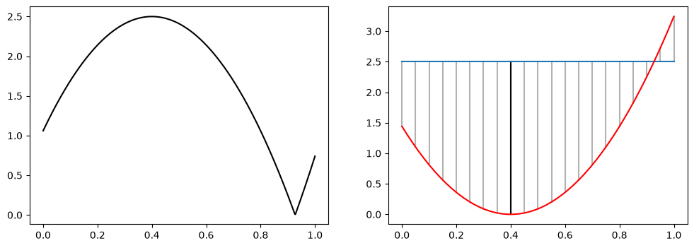
For example, if we want to compute the distance between the functions $f$ and $g$ defined on the interval $[0,1]$ such that $f(x)=(x-0.4)^2$ and $g(x) = 2.5$, we have to find the value that maximizes the function $h(x) = | (x-0.4)^2 - 2.5|$, plotted in the first image of the figure below. This is not always an easy task, since we have no assumption about the differentiability of our functions, and the absolute value makes it even harder by creating new peaks. In the second image of the figure below we have a visual interpretation of what we want. The value of the distance will be the place where the curves are farthest apart.
Por exemplo, se queremos calcular a distância entre as funções $f$ e $g$ definidas no intervalo $[0,1]$ tais que $f(x)=(x-0.4)^2$ e $g(x) = 2.5$, temos que achar o valor que maximiza a função $h(x) = | (x-0.4)^2 - 2.5|$, plotada na primeira imagem da figura abaixo. Isso nem sempre é uma tarefa fácil, pois não temos nenhuma hipótese sobre a diferenciabilidade das nossas funções e o módulo atrapalha ainda mais criando novos picos. Na segunda imagem da figura abaixo temos uma interpretação visual do que queremos. O valor da distância será o local em que as curvas estão mais distantes.
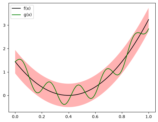
In this metric, the ball of radius $r>0$ around the function $f:[a,b]\to\mathbb{R}$ is all the functions (defined on the interval $[a,b]$) that always stay within the band around $f$ of width $2r$. In the figure below we have an example of this. The function $g(x) = (x-0.4)^2 + 0.4\sin(30x)$ is inside the ball $B_{d_{\max}}((x-0.4)^2;0.5)$ since the distance between them is $\max_{x\in[0,1]} |0.4 \sin(30x) |=0.4<0.5$.
Nessa métrica, a bola de raio $r>0$ ao redor da função $f:[a,b]\to\mathbb{R}$ são todas as funções (definidas no intervalo $[a,b]$) que ficam sempre dentro da faixa ao redor de $f$ de largura $2r$. Na figura abaixo temos um exemplo disso. A função $g(x) = (x-0.4)^2 + 0.4\sin(30x)$ está dentro da bola $B_{d_{\max}}((x-0.4)^2;0.5)$ pois a distância entre elas é $\max_{x\in[0,1]} |0.4 \sin(30x) |=0.4<0.5$.
$\oint$ The KS test uses a variation of this metric to define a distance between random variables based on the distance between their cumulative distribution functions.
$\oint$ O teste KS usa uma variação dessa métrica pra definir uma distância entre variáveis aleatórias a partir da distância entre as funções densidade acumulada.
Weighted distance
Distância Ponderada
In many cases it can be important to assign a greater weight to one of the coordinates, giving rise to the idea of the weighted distance. For example, if $\mathcal{A}=\mathbb{R}^2$ and being close in the first coordinate is $10$ times more important than being close in the second, we can make a variation of the euclidean metric to compute the distance between $\textbf{x} = (x_1,x_2)$ and $\textbf{y}=(y_1,y_2)$ as
Em muitos casos pode ser importante atribuir um peso maior para alguma das coordenadas, surgindo a ideia da distância ponderada. Por exemplo, se $\mathcal{A}=\mathbb{R}^2$ e estar perto na primeira coordenada é $10$ vezes mais importante do que estar perto na segunda, podemos fazer uma variação da métrica Euclidiana para calcular a distância entre $\textbf{x} = (x_1,x_2)$ e $\textbf{y}=(y_1,y_2)$ como
\[\begin{equation*} d_{\textrm{weighted}}(\textbf{x},\textbf{y}) = \sqrt{10 (x_1-y_1)^2 +(x_2-y_2)^2 }\,. \end{equation*}\]
\[\begin{equation*} d_{\textrm{ponderada}}(\textbf{x},\textbf{y}) = \sqrt{10 (x_1-y_1)^2 +(x_2-y_2)^2 }\,. \end{equation*}\]
We will not go into details, but we can do this whenever we have a positive-definite matrix $A$, by defining
Não entraremos em detalhes, mas podemos fazer isso sempre que temos uma matriz $A$ positiva definida definindo
\[\begin{equation*} d_{\textrm{weighted}}(\textbf{x},\textbf{y}) = \sqrt{(\textbf{x}-\textbf{y})^T \, A \,(\textbf{x}-\textbf{y}) }\,, \end{equation*}\]
\[\begin{equation*} d_{\textrm{ponderada}}(\textbf{x},\textbf{y}) = \sqrt{(\textbf{x}-\textbf{y})^T \, A \,(\textbf{x}-\textbf{y}) }\,, \end{equation*}\]
performing the usual multiplication operations of row vectors, column vectors, and matrices. Therefore, with $A$ fixed, we can implement this metric to use the
open_ball function as we did with the discrete metric.fazendo as operações usuais de multiplicação de vetores linha, coluna e matrizes. Portanto, fixada $A$, podemos implementar essa métrica para usar a função
open_ball como fizemos com a métrica discreta.def weighted(X, Y):
"""Weighted distance between X and Y for a positive-definite matrix A."""
return np.dot(X - Y, np.matmul(A, X - Y))
A matrix with all positive diagonal values is always a positive-definite matrix. In this case we can interpret the diagonal values as the weights we want to give to each of the coordinates. The usual euclidean distance occurs when $A$ is the identity matrix. The case studied earlier occurs when
Uma matriz com todos valores da diagonal positivos é sempre uma matriz positiva definida. Neste caso podemos interpretar os valores da diagonal como os pesos que queremos dar em cada uma das coordenadas. A distância euclidiana usual ocorre quando $A$ é a matriz identidade. Já o caso estudado anteriormente ocorre quando
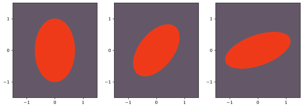
We can play with these different matrices by placing weights on the coordinates we consider most important. Values off the main diagonal can be interpreted as an interaction between those coordinates. They will distort the shape of the ball, as we can see below, where we have, respectively, the positive-definite matrices
Podemos brincar com essas diferentes matrizes colocando pesos nas coordenadas que consideramos mais importantes. Valores fora da diagonal principal podem ser interpretados como uma interação entre aquelas coordenadas. Eles vão distorcer o formato da bola, como podemos ver abaixo em que temos, respectivamente, as matrizes positivas definidas
\[A= \left[\begin{array}{cc} 2 & 0 \\ 0 & 1 \end{array}\right], \left[\begin{array}{cc} 2 & -1 \\ -1 & 2 \end{array}\right]\textrm{, and }\left[\begin{array}{cc} 1 & -1 \\ -1 & 4 \end{array}\right].\]
\[A= \left[\begin{array}{cc} 2 & 0 \\ 0 & 1 \end{array}\right], \left[\begin{array}{cc} 2 & -1 \\ -1 & 2 \end{array}\right]\textrm{, e }\left[\begin{array}{cc} 1 & -1 \\ -1 & 4 \end{array}\right].\]
Explainability by reference
Explicabilidade por referência
The notion of distance is a very important concept. It is an intuitive way of giving us a notion of similarity (and dissimilarity) between examples. In the supervised learning context, if your way of computing distance is reasonably understandable, models that work by finding nearby neighbors become explainable by reference. If we want to understand why it gave a certain prediction for an example, we look at the training data similar to the observation we are evaluating.
A noção de distância é um conceito muito importante. Ela é um jeito intuitivo de nos dar uma noção de similaridade (e dissimilaridade) entre exemplos. No contexto de aprendizado supervisionado, se sua forma de calcular distância é razoavelmente compreensível, modelos que funcionam através de encontrar vizinhos próximos tornam-se explicáveis por referência. Se queremos entender o motivo dele ter dado determinada previsão para um exemplo, olhamos para os dados do treino parecidos com a observação que estamos avaliando.
To put it in an example, suppose we have a binary classification problem in which we are trying to predict whether a client is a defaulter or not. Using strategies that find nearby neighbors in the training set gives us explanations for the answer for a given client. We are looking at clients with similar attributes (according to our distance) and making the prediction from them. If we want to know why a given client was considered a defaulter, we look at the nearest neighbors and understand why the model gave the result it gave.
Colocando em um exemplo, suponha que temos um problema de classificação binária em que estamos tentando prever se um cliente é inadimplente ou não. Usar estratégias que encontram vizinhos próximos na base de treinamento nos dá explicações para a resposta de um determinado cliente. Estamos olhando clientes com atributos parecidos (segundo nossa distância) e fazendo a previsão a partir deles. Se queremos saber por que um determinado cliente foi considerado inadimplente, olhamos para os vizinhos mais próximos e entendemos por que o modelo deu o resultado que deu.
I hope this post, which was a lot of fun to write, has been useful for better understanding what distance means and the differences between distances. At the very least, you can now use some of the metrics we discussed here as one of the hyperparameters of your distance-based models!
Espero que este post, muito divertido de escrever, tenha sido útil para entender melhor o que significa distância e as diferenças entre elas. No mínimo, agora você pode usar algumas das métricas que discutimos aqui como um dos hiper-parâmetros dos seus modelos baseados em distância!
$\oint$ The swap is not always immediate. In K-Means, for example, the update of the centroids is the mean of the examples in that cluster precisely because the mean minimizes the cost function given by the sum of the euclidean distances from the examples to their respective centroids. If we choose to minimize the sum of the Minkowski distances with parameter 1 (L1), then the update of the centroids is done with the coordinate-wise median, since these are the values that minimize the modified cost function; this is K-Medians.
$\oint$ Nem sempre a troca é imediata. No K-Means, por exemplo, a atualização dos centroides é a média dos exemplos daquele cluster justamente porque a média minimiza a função custo dada pela soma das distâncias euclidianas dos exemplos até os seus respectivos centroides. Se escolhemos minimizar a soma das distâncias de Minkowski de parâmetro 1 (L1), então a atualização dos centroides é feita com a mediana coordenada a coordenada uma vez que estes são os valores que minimizam a função de custo alterada, este é o K-Medians.
You can find all the code and the environment needed to reproduce the experiments in the repository of this post.
Você pode encontrar todos os códigos e o ambiente necessário para reproduzir os experimentos no repositório deste post.