Covariate Shift: Introduction

The primary goal of supervised learning is to identify patterns between independent variables (explanatory variables) and a dependent variable (target variable). In mathematical terms, within a regression context, we have a random vector $V = (X_1, X_2, \cdots, X_n, Y)$ and we suppose that there exists a relationship between the independent variables $X_i$ and the dependent variable $Y$, expressed as:

O principal objetivo do aprendizado supervisionado é tentar reconhecer padrões entre variáveis explicativas e uma variável alvo. Matematicamente, no caso da regressão, temos um vetor aleatório $V = (X_1, X_2, \cdots, X_n, Y)$ e supomos que existe uma relação entre as variáveis explicativas $X_i$ e a variável alvo $Y$ do tipo

\[\left(Y \,|\, X_1=x_1, X_2=x_2,\cdots, X_n=x_n\right)\sim f(x_1, x_2,\cdots, x_n) + \varepsilon,\]

where $f:\mathbb{R}^n\to \mathbb{R}$ is any given function and $\varepsilon$ is a random variable with mean $0$, referred to as noise (which might also vary depending on the values of $X_i$). The supervised learning approach attempts to estimate the function $f$ using prior observations (a sample of the random vector $V$).

onde $f:\mathbb{R}^n\to \mathbb{R}$ é uma função qualquer e $\varepsilon$ é uma variável aleatória com média $0$ chamada de ruído (que possivelmente pode mudar dependendo dos valores de $X_i$ também). O paradigma de aprendizado supervisionado tenta estimar a função $f$ com observações anteriores (uma amostra do vetor aleatório $V$).

$\oint$ Note that our illustration uses regression as an example due to its straightforwardness. Nonetheless, the case of classification isn't significantly more complex. In binary classification, the aim is to estimate $f:\mathbb{R}^n\to [0,1]$ as follows:

$\oint$ Ainda que estejamos exemplificando com o problema de regressão por ser mais imediato, o caso de classificação não é muito mais sofisticado. Na classificação binária, estamos interessados em estimar $f:\mathbb{R}^n\to [0,1]$ tal que:

\[\left(Y \,|\, X_1=x_1, X_2=x_2,\cdots, X_n=x_n\right)\sim \textrm{Bernoulli}(p)\textrm{, with }p=f(x_1, x_2,\cdots, x_n).\]

Generally, during cross-validation, we expect that the performance of our estimated function will remain consistent on the validation set when faced with new data. Machine learning in non-stationary environments, however, presents a challenge: What happens if there's a dataset shift, meaning the distribution of the random vector $V$ differs in new data? Can we realistically expect the model to uphold its validated performance?

Em geral, quando fazemos uma validação cruzada, esperamos que o desempenho da nossa função estimada continue sendo o mesmo que no conjunto de validação quando o modelo se deparar com dados novos. O problema de aprendizado de máquina em ambientes não-estacionários traz novos desafios ao nosso trabalho: e se houver um dataset shift, isto é, e se a distribuição do vetor aleatório $V$ for diferente nos dados que ainda não conhecemos? É razoável esperar que o modelo mantenha o desempenho obtido na validação?

In this context, we encounter two common scenarios [1]. The first, concept shift, takes place when the function $f$ connecting the variables $X_i$ and $Y$ changes. A seemingly less noticeable but equally alarming issue arises when the relationship between the explanatory and target variables remains constant, but the distribution of variables $X_i$ in new examples deviates from the distribution in the training data. This is known as covariate shift, a situation that we'll learn to identify and offer a potential solution for in this series of posts.

Dentro desse contexto há pelo menos duas variações clássicas <a href=#bibliography>[1]</a>. A primeira é o concept shift, que ocorre quando a função $f$ que relaciona as variáveis $X_i$ e $Y$ muda. Um problema aparentemente mais sutil, mas igualmente apavorante é o caso em que a relação entre as variáveis explicativas e a variável alvo é conservada, mas a distribuição das variáveis $X_i$ nos novos exemplos é diferente da distribuição das variáveis $X_i$ nos dados de treinamento. Esse é o covariate shift, situação que vamos aprender a identificar nesta série de posts e dar uma possível abordagem de solução.

But first, let's create an artificial scenario that exhibits covariate shift. This will help illuminate the concepts through a practical situation and explore the problems that may emerge if this shift isn't properly identified and addressed.

Antes, vamos construir artificialmente um cenário que apresenta covariate shift para esclarecer as ideias com uma situação prática, e analisar o problema que surge caso isso não seja identificado e tratado adequadamente.

Example of dataset shift between training data and production data

Exemplo de dataset shift entre dados de treino e dados de produção

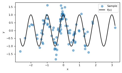
Consider $X$ to be a random variable that follows a normal distribution, $X\sim \mathcal{N}(0,1)$. Let $f:\mathbb{R}\to\mathbb{R}$ be a function defined as $f(x) = \cos(2\pi x)$, and $\varepsilon$ be a noise variable modeled as $\varepsilon \sim \mathcal{N}(0,0.25)$. We will build a dataset generated by this random experiment.

Sejam $X$ uma variável aleatória tal que $X\sim \mathcal{N}(0,1)$, $f:\mathbb{R}\to\mathbb{R}$ uma função da forma $f(x) = \cos(2\pi x)$ e $\varepsilon$ é um ruído modelado como $\varepsilon \sim \mathcal{N}(0,0.25)$. Construiremos um conjunto de dados gerados por esse experimento aleatório.

def f(X):
    return np.cos(2 * np.pi * X)

def f_ruido(X, random_state):
    return f(X) + np.random.RandomState(random_state).normal(0, 0.5, size=X.shape[0])

def sample(n, mean=0, random_state=None):
    rs = np.random.RandomState(random_state).randint(
        0, 2**32 - 1, dtype=np.int64, size=2
    )
    X = np.random.RandomState(rs[0]).normal(mean, 1, size=n)
    Y = f_ruido(X, random_state=rs[1])
    return X.reshape(-1, 1), Y.reshape(-1, 1)

In this example, we will conduct this experiment $100$ times, creating our data with the mean of $X$ at $0$ as previously mentioned.

Neste exemplo, faremos este experimento $100$ vezes, criando nossos dados com a média de $X$ em $0$ como comentado anteriormente.

Despite the noise being of the same order of magnitude as $f$, the pattern of the function that drives the generation of the data can still be discerned. Our goal is to make predictions: given new observations of $X=x$, we aim to estimate the corresponding values for $(Y \, | \, X=x)$.

Apesar do ruído ser da ordem de grandeza $f$, é possível visualizar o padrão da função que guia a geração dos dados. Estamos interessados em fazer previsões: dadas novas observações de $X=x$, queremos estimar os respectivos valores para $(Y \, | \, X=x)$.

X_past, Y_past = sample(100, random_state=42)

x_plot = np.linspace(np.min(X_past), np.max(X_past), 1000).reshape(-1, 1)

fig, ax = plt.subplots(figsize=(5, 3))
ax.scatter(X_past, Y_past, alpha=0.5, label="Sample")
ax.plot(x_plot, f(x_plot), c="k", label="f(x)")
ax.set_xlabel("x")
ax.set_ylabel("y")
ax.legend()
plt.tight_layout()

We will employ a simple model for regression, namely the sklearn.tree.DecisionTreeRegressor. By using sklearn.model_selection.GridSearchCV, we can determine the optimal value for the minimum number of samples per leaf (a regularization parameter, intended to prevent overfitting). Based on cross-validation, we can estimate the potential value of sklearn.metrics.r2_score we might achieve if we applied the decision tree to unseen data.

Usaremos um modelo simples para fazer a regressão, o sklearn.tree.DecisionTreeRegressor. Com um sklearn.model_selection.GridSearchCV, escolhemos o melhor valor para o mínimo de exemplos por folha (parâmetro de regularização, evitando overfit). Com base na validação cruzada, estimamos o valor de sklearn.metrics.r2_score que seria obtido se utilizássemos a árvore em dados nunca antes vistos.

from sklearn.tree import DecisionTreeRegressor
from sklearn.model_selection import GridSearchCV

dtr = DecisionTreeRegressor(random_state=42)
param = {"min_samples_leaf": np.arange(1, 10, 1)}
grid_search = GridSearchCV(
    dtr, param, cv=5, scoring="r2", return_train_score=True
).fit(X_past, Y_past)

df_cv = (
    pd.DataFrame(grid_search.cv_results_)
    .sort_values("rank_test_score")
    .filter(["param_min_samples_leaf", "mean_test_score", "std_test_score"])
)
df_cv.head(3)

	param_min_samples_leaf	mean_test_score	std_test_score
2	3	0.554561	0.094576
6	7	0.502175	0.100091
3	4	0.490702	0.131177

We attain a reasonable $R^2$ value, indicating that the model successfully captures the patterns in the data, despite its simplicity and the small size of the dataset.

Obtemos um $R^2$ razoável, demonstrando que há um aprendizado dos padrões dos dados (apesar de ser um modelo simples e termos poucos exemplos).

fig, ax = plt.subplots(figsize=(5, 3))
ax.scatter(X_past, Y_past, alpha=0.6, label="Sample")
ax.plot(x_plot, f(x_plot), c="k", alpha=0.5, label="f(x)")
ax.plot(
    x_plot,
    grid_search.best_estimator_.predict(x_plot),
    c="r",
    label="Decision tree estimator",
)
ax.set_xlabel("x")
ax.set_ylabel("y")
ax.legend()
plt.tight_layout()

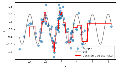
Visually, the model performs well around $x=0$, where there's a high density of $x$ values. As expected, the model's performance deteriorates at the fringes where fewer training examples are present.

Graficamente, vemos que o modelo faz um bom trabalho ao redor do $x=0$, onde temos uma concentração de valores de $x$, e, naturalmente, perde a qualidade nas bordas, onde há menos exemplos de treinamento.

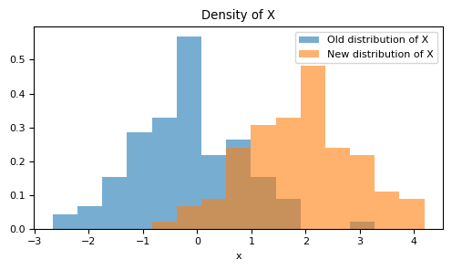
Let's now imagine a scenario where circumstances have changed: the relationship between $X$ and $Y$ remains intact, but for some reason, the distribution of the variable $X$ is no longer $X\sim \mathcal{N}(0,1)$. Instead, it's given by $X\sim \mathcal{N}(2,1)$. In other words, there's a shift in the distribution.

Imaginemos agora que o cenário mudou: apesar da relação entre $X$ e $Y$ continuar sendo a mesma, por algum motivo, a variável $X$ não tem mais distribuição dada por $X\sim \mathcal{N}(0,1)$. Nesta variação, ela é dada por $X\sim \mathcal{N}(2,1)$, ou seja, temos uma translação da distribuição.

X_new, Y_new = sample(100, mean=2, random_state=13)

min_X = np.min(np.vstack([X_past, X_new]))
max_X = np.max(np.vstack([X_past, X_new]))

fig, ax = plt.subplots(figsize=(5, 3))
ax.hist(
    X_past,
    alpha=0.6,
    bins=np.linspace(min_X, max_X, 16),
    density=True,
    label="Old distribution of X",
)
ax.hist(
    X_new,
    alpha=0.6,
    bins=np.linspace(min_X, max_X, 16),
    density=True,
    label="New distribution of X",
)
ax.set_xlabel("x")
ax.set_title("Density of X")
ax.legend()
plt.tight_layout()

It is not reasonable to expect that our model will maintain the same performance as before. The estimation of the sklearn.metrics.r2_score was made based on the original distribution of $X$, which has now shifted.

Não é razoável esperar que o nosso modelo continue com a mesma performance que tínhamos anteriorente. A estimação do sklearn.metrics.r2_score estava sendo feita na distribuição antiga de $X$ e agora mudamos ela.

$\oint$ We will delve into this in more depth in a future post in this series, but essentially, the previous model was trained to identify a function $h$ that minimizes the expected squared error in the distribution $(X_{\textrm{old}}, Y)$. Mathematically, this can be represented as:

$\oint$ Vamos explorar isso com mais detalhe em um post futuro dessa série, mas o modelo anterior estava sendo treinado para achar uma função $h$ tal que

\[h* = \arg\min_{h\in\mathcal{H}}\,\mathbb{E}_{(X_{\textrm{old}}, Y)} \left(\left(h(X) - Y\right)^2\right),\]

This was done approximately, using the sample, by computing the empirical mean squared error. However, now, we are dealing with new data. Ideally, we should be minimizing:

Ou seja, uma hipótese $h$ que minimize a esperança do erro quadrático na distribuição $(X_{\textrm{old}}, Y)$. Isso é feito de forma aproximada, com a amostra observada, calculando o erro quadrático médio empírico. De qualquer forma, agora, estamos olhando para novos dados. O ideal seria minimizar

\[\mathbb{E}_{(X_{\textrm{new}}, Y)} \left(\left(h(X) - Y\right)^2\right).\]

That is, we are targeting the expected error in a different distribution.

Ou seja, uma esperança de uma distribuição diferente.

from sklearn.metrics import r2_score

x_plot_new = np.linspace(min_X, max_X, 1000).reshape(-1, 1)

fig, ax = plt.subplots(figsize=(7, 3))
ax.scatter(X_past, Y_past, alpha=0.2, label="Old sample")
ax.scatter(X_new, Y_new, alpha=0.6, label="New sample")
ax.plot(x_plot_new, f(x_plot_new), c="k", alpha=0.2, label="f(x)")
ax.plot(
    x_plot_new,
    grid_search.best_estimator_.predict(x_plot_new),
    c="r",
    label="Decision tree estimator trained on old sample",
)
ax.set_xlabel("x")
ax.set_ylabel("y")
ax.legend(loc="lower left")
plt.tight_layout()

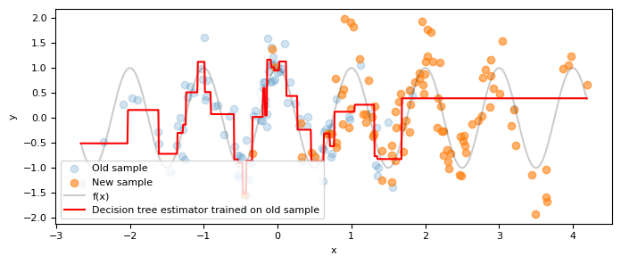
r2_score(Y_new, grid_search.best_estimator_.predict(X_new))

0.059081313039643146

As anticipated, the model's performance deteriorates when applied to the new data. It's important to remember that the relationship between $Y$ and $X$ has remained the same; only the distribution of $X$ has shifted.

Como esperado, a qualidade do modelo cai nos dados novos. Lembrando que a relação $Y\,|\,X$ não mudou, apenas a distribuição de $X$.

Identifying covariate shift

Identificando covariate shift

With the initial problem established, our challenge can be summarized as follows:

Dada a motivação inicial, temos um desafio resumido no seguinte enunciado:

Let $X$ and $Z$ be random variables (or vectors). Assume you independently sample $X$ $N\in\mathbb{N}^*$ times and $Z$ $M\in \mathbb{N}^*$ times, resulting in the samples $\{x_1, x_2, \cdots, x_N \} $ and $\{z_1, z_2, \cdots, z_M \} $. How can we determine if $X\sim Z$ using only these two samples? Specifically, in the context of covariate shift, we'll be comparing samples of covariates from the training phase with those in production.

Seja $X$ e $Z$ variáveis (ou vetores) aleatórias. Suponha que amostre $X$ de forma independente $N\in\mathbb{N}^*$ vezes e também $Z$ seja amostrada também de forma independente $M\in \mathbb{N}^*$ vezes ficando com as amostras $\{x_1, x_2, \cdots, x_N \} $ e $\{z_1, z_2, \cdots, z_M \} $. Como saber se $X\sim Z$ olhando apenas para as duas amostras? No contexto específico do covariate shift, vamos estar comparando as amostras das covariáveis no treino e depois em produção.

In general, monitoring the distribution of covariates needs to be easy to implement. Simple methods are preferred over complex ones to prioritize computational efficiency. Moreover, analysis is typically performed on each covariate, identifying shifts in these marginal distributions. Among the classic univariate methods, the most prominent are:

No geral, o monitoramento da distribuição das covariáveis precisa ser simples. Métodos básicos são escolhidos no lugar de técnicas complexas privilegiando eficiência computacional. Além disso, a análise costuma ser feita olhando covariável por covariável, identificando mudanças nessas distribuições marginais. Entre os métodos clássicos univariados, se destacam:

Comparison of statistics: means, variances, select sample quantiles etc;

Comparação de estatísticas: médias, variâncias e alguns quantis amostrais;

Comparison of frequencies for discrete distributions and categorical data;

Comparação de frequências para distribuições discretas e dados categóricos;

Kolmogorov-Smirnov test;

Teste de Kolmogorov-Smirnov;

Kullback-Leibler divergence.

Divergência de Kullback-leibler.

This monitoring is often accompanied by analysis of the model's output distribution. For instance, if our model previously suggested that 10% of the data belonged to one class, and now it indicates 20%, we have a solid hint that the input distribution has shifted.

Muitas vezes esse monitoramento é feito aliado à análise da distribuição da saída do modelo. Se antes o nosso modelo indicava que 10% dos dados eram de uma classe e agora ele diz que 20% são daquela classe, temos um bom indicativo de que a distribuição de entrada mudou.

In this series of posts, I plan to introduce some slightly more unconventional methods for identifying covariate shift. Subsequently, we'll explore the problem through Vapnik's empirical risk minimization framework. From there, we'll derive an elegant method to address it, using a technique that will serve as a diagnostic tool for identifying dataset shift.

Nesta série de postagens pretendo apresentar alguns métodos um pouco mais alternativos para identificar o covariate shift. Em seguida, vamos entender porque ele ocorre sob a luz da minimização do risco empírico de Vapnik. Derivaremos uma maneira muito elegante de tratá-lo a partir de uma técnica que será um diagnóstico para identificação do dataset shift.

$\oint$ Keep in mind that this is just one of the crucial elements when it comes to monitoring machine learning models. For a comprehensive guide that addresses the main potential issues, I recommend the references [2, 3].

$\oint$ Lembre-se que dataset shift é apenas um dos elementos cruciais quando se trata de monitorar modelos de aprendizado de máquina. Para um guia completo que aborda as principais questões potenciais, sugiro as referências <a href=#bibliography>[2, 3]</a>.