Este texto foi inicialmente redigido em português e posteriormente traduzido. A versão original em português pode ser encontrada no repositório de experimentos.
The primary goal of supervised learning is to identify patterns between independent variables (explanatory variables) and a dependent variable (target variable). In mathematical terms, within a regression context, we have a random vector $V = (X_1, X_2, \cdots, X_n, Y)$ and we suppose that there exists a relationship between the independent variables $X_i$ and the dependent variable $Y$, expressed as:
\[\left(Y \,|\, X_1=x_1, X_2=x_2,\cdots, X_n=x_n\right)\sim f(x_1, x_2,\cdots, x_n) + \varepsilon,\]where $f:\mathbb{R}^n\to \mathbb{R}$ is any given function and $\varepsilon$ is a random variable with mean $0$, referred to as noise (which might also vary depending on the values of $X_i$). The supervised learning approach attempts to estimate the function $f$ using prior observations (a sample of the random vector $V$).
$\oint$ Note that our illustration uses regression as an example due to its straightforwardness. Nonetheless, the case of classification isn't significantly more complex. In binary classification, the aim is to estimate $f:\mathbb{R}^n\to [0,1]$ as follows:
\[\left(Y \,|\, X_1=x_1, X_2=x_2,\cdots, X_n=x_n\right)\sim \textrm{Bernoulli}(p)\textrm{, com }p=f(x_1, x_2,\cdots, x_n).\]Generally, during cross-validation, we expect that the performance of our estimated function will remain consistent on the validation set when faced with new data. Machine learning in non-stationary environments, however, presents a challenge: What happens if there's a dataset shift, meaning the distribution of the random vector $V$ differs in new data? Can we realistically expect the model to uphold its validated performance?
In this context, we encounter two common scenarios [1]. The first, concept shift, takes place when the function $f$ connecting the variables $X_i$ and $Y$ changes. A seemingly less noticeable but equally alarming issue arises when the relationship between the explanatory and target variables remains constant, but the distribution of variables $X_i$ in new examples deviates from the distribution in the training data. This is known as covariate shift, a situation that we'll learn to identify and offer a potential solution for in this series of posts.
But first, let's create an artificial scenario that exhibits covariate shift. This will help illuminate the concepts through a practical situation and explore the problems that may emerge if this shift isn't properly identified and addressed.
Example of dataset shift between training data and production data
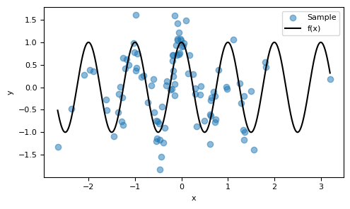
Consider $X$ to be a random variable that follows a normal distribution, $X\sim \mathcal{N}(0,1)$. Let $f:\mathbb{R}\to\mathbb{R}$ be a function defined as $f(x) = \cos(2\pi x)$, and $\varepsilon$ be a noise variable modeled as $\varepsilon \sim \mathcal{N}(0,0.25)$. We will build a dataset generated by this random experiment.
def f(X):
    return np.cos(2 * np.pi * X)

def f_ruido(X, random_state):
    return f(X) + np.random.RandomState(random_state).normal(0, 0.5, size=X.shape[0])

def sample(n, mean=0, random_state=None):
    rs = np.random.RandomState(random_state).randint(
        0, 2**32 - 1, dtype=np.int64, size=2
    )
    X = np.random.RandomState(rs[0]).normal(mean, 1, size=n)
    Y = f_ruido(X, random_state=rs[1])
    return X.reshape(-1, 1), Y.reshape(-1, 1)
In this example, we will conduct this experiment $100$ times, creating our data with the mean of $X$ at $0$ as previously mentioned.
Despite the noise being of the same order of magnitude as $f$, the pattern of the function that drives the generation of the data can still be discerned. Our goal is to make predictions: given new observations of $X=x$, we aim to estimate the corresponding values for $(Y \, | \, X=x)$.
X_past, Y_past = sample(100, random_state=42)

x_plot = np.linspace(np.min(X_past), np.max(X_past), 1000).reshape(-1, 1)

fig, ax = plt.subplots(figsize=(5, 3))
ax.scatter(X_past, Y_past, alpha=0.5, label="Sample")
ax.plot(x_plot, f(x_plot), c="k", label="f(x)")
ax.set_xlabel("x")
ax.set_ylabel("y")
ax.legend()
plt.tight_layout()
We will employ a simple model for regression, namely the
sklearn.tree.DecisionTreeRegressor. By using sklearn.model_selection.GridSearchCV, we can determine the optimal value for the minimum number of samples per leaf (a regularization parameter, intended to prevent overfitting). Based on cross-validation, we can estimate the potential value of sklearn.metrics.r2_score we might achieve if we applied the decision tree to unseen data.from sklearn.tree import DecisionTreeRegressor
from sklearn.model_selection import GridSearchCV
dtr = DecisionTreeRegressor(random_state=42)
param = {"min_samples_leaf": np.arange(1, 10, 1)}
grid_search = GridSearchCV(
dtr, param, cv=5, scoring="r2", return_train_score=True
).fit(X_past, Y_past)
df_cv = (
pd.DataFrame(grid_search.cv_results_)
.sort_values("rank_test_score")
.filter(["param_min_samples_leaf", "mean_test_score", "std_test_score"])
)
df_cv.head(3)
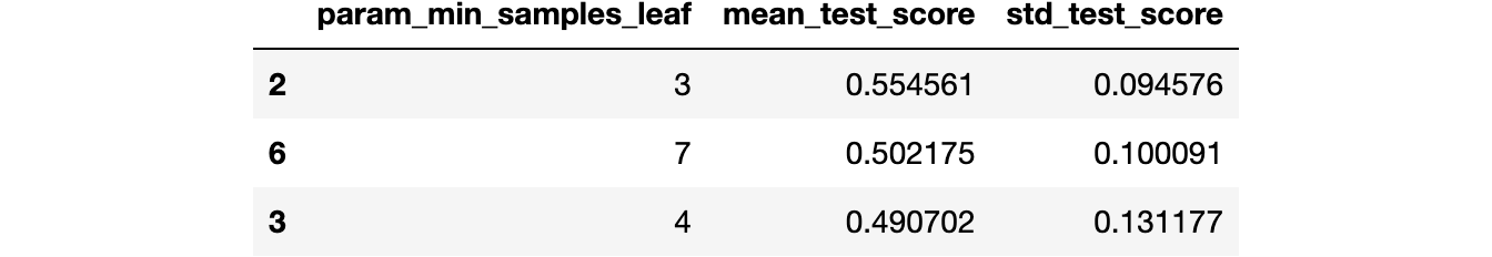
We attain a reasonable $R^2$ value, indicating that the model successfully captures the patterns in the data, despite its simplicity and the small size of the dataset.
fig, ax = plt.subplots(figsize=(5, 3))
ax.scatter(X_past, Y_past, alpha=0.6, label="Sample")
ax.plot(x_plot, f(x_plot), c="k", alpha=0.5, label="f(x)")
ax.plot(
    x_plot,
    grid_search.best_estimator_.predict(x_plot),
    c="r",
    label="Decision tree estimator",
)
ax.set_xlabel("x")
ax.set_ylabel("y")
ax.legend()
plt.tight_layout()
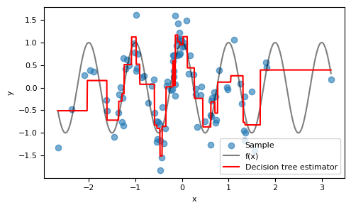
Visually, the model performs well around $x=0$, where there's a high density of $x$ values. As expected, the model's performance deteriorates at the fringes where fewer training examples are present.
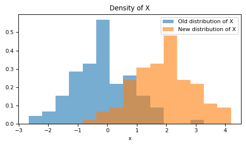
Let's now imagine a scenario where circumstances have changed: the relationship between $X$ and $Y$ remains intact, but for some reason, the distribution of the variable $X$ is no longer $X\sim \mathcal{N}(0,1)$. Instead, it's given by $X\sim \mathcal{N}(2,1)$. In other words, there's a shift in the distribution.
X_new, Y_new = sample(100, mean=2, random_state=13)

min_X = np.min(np.vstack([X_past, X_new]))
max_X = np.max(np.vstack([X_past, X_new]))

fig, ax = plt.subplots(figsize=(5, 3))
ax.hist(
    X_past,
    alpha=0.6,
    bins=np.linspace(min_X, max_X, 16),
    density=True,
    label="Old distribution of X",
)
ax.hist(
    X_new,
    alpha=0.6,
    bins=np.linspace(min_X, max_X, 16),
    density=True,
    label="New distribution of X",
)
ax.set_xlabel("x")
ax.set_title("Density of X")
ax.legend()
plt.tight_layout()
It is not reasonable to expect that our model will continue with the same performance we had before. The estimation of the
sklearn.metrics.r2_score was made based on the original distribution of $X$, which has now shifted.$\oint$ We will delve into this in more depth in a future post in this series, but essentially, the previous model was trained to identify a function $h$ that minimizes the expected squared error in the distribution $(X_{\textrm{old}}, Y)$. Mathematically, this can be represented as:
\[h* = \arg\min_{h\in\mathcal{H}}\,\mathbb{E}_{(X_{\textrm{old}}, Y)} \left(\left(h(X) - Y\right)^2\right),\]This was done approximately, using the sample, by computing the empirical mean squared error. However, now, we are dealing with new data. Ideally, we should be minimizing:
\[\mathbb{E}_{(X_{\textrm{new}}, Y)} \left(\left(h(X) - Y\right)^2\right).\]That is, we are targeting the expected error in a different distribution.
from sklearn.metrics import r2_score

x_plot_new = np.linspace(min_X, max_X, 1000).reshape(-1, 1)

fig, ax = plt.subplots(figsize=(7, 3))
ax.scatter(X_past, Y_past, alpha=0.2, label="Old sample")
ax.scatter(X_new, Y_new, alpha=0.6, label="New sample")
ax.plot(x_plot_new, f(x_plot_new), c="k", alpha=0.2, label="f(x)")
ax.plot(
    x_plot_new,
    grid_search.best_estimator_.predict(x_plot_new),
    c="r",
    label="Decision tree estimator trained on old sample",
)
ax.set_xlabel("x")
ax.set_ylabel("y")
ax.legend(loc="lower left")
plt.tight_layout()
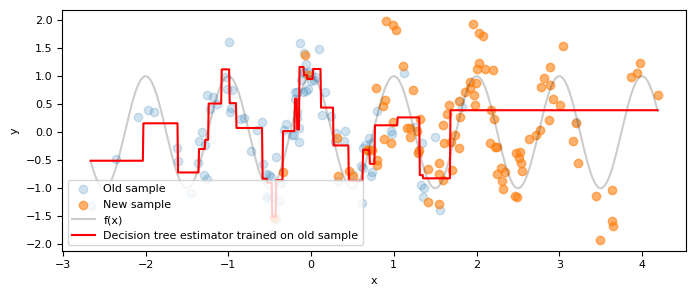
r2_score(Y_new, grid_search.best_estimator_.predict(X_new))
0.059081313039643146
As anticipated, the model's performance deteriorates when applied to the new data. It's important to remember that the relationship between $Y$ and $X$ has remained the same; only the distribution of $X$ has shifted.
Identifying covariate shift
With the initial problem established, our challenge can be summarized as follows:
Let $X$ and $Z$ be random variables (or vectors). Assume you independently sample $X$ $N\in\mathbb{N}^*$ times and $Z$ $M\in \mathbb{N}^*$ times, resulting in the samples $\{x_1, x_2, \cdots, x_N \} $ and $\{z_1, z_2, \cdots, z_M \} $. How can we determine if $X\sim Z$ using only these two samples? Specifically, in the context of covariate shift, we'll be comparing samples of covariates from the training phase with those in production.
In general, monitoring the distribution of covariates needs to be easy to implement. Simple methods are preferred over complex ones to prioritize computational efficiency. Moreover, analysis is typically performed on each covariate, identifying shifts in these marginal distributions. Among the classic univariate methods, the most prominent are:
- Comparison of statistics: means, variances, select sample quantiles etc;
- Comparison of frequencies for discrete distributions and categorical data;
- Kolmogorov-Smirnov test;
- Kullback-Leibler divergence.
This monitoring often occurs with the analysis of the model's output distribution. For instance, if our model previously suggested that 10% of the data belonged to one class, and now it indicates 20%, we have a solid hint that the input distribution has shifted.
In this series of posts, I plan to introduce some slightly more unconventional methods for identifying covariate shift. Subsequently, we'll explore the problem through Vapnik's empirical risk minimization framework. From there, we'll derive an elegant method to address it, using a technique that will serve as a diagnostic tool for identifying dataset shift.
$\oint$ Keep in mind that this is just one of the crucial elements when it comes to monitoring machine learning models. For a comprehensive guide that addresses the main potential issues, I recommend the references [2, 3].
Bibliography
[3] A Guide to Monitoring Machine Learning Models in Production. NVIDIA Developer Blog. Kurtis Pykes.
You can find all files and environments for reproducing the experiments in the repository of this post.